3. Meshes in Monocurl
We'll now talk about meshes, the objects that we see on screen. This section is a bit long, but a lot of it is just examples. The optional sections discuss some of the decisions behind Monocurl, but are not that practical so feel free to skim them.
3.1 Following Along
In this section, you finally have many opportunities to follow along!
Simply create a new scene in the Monocurl editor, and in the slide_1 section, add the required code for creating the meshes.
We haven't officially discussed animations yet, but for now you'll have to use the following lines to show the meshes we create. You might also want to change the background to WHITE for some scenes with black meshes.
tree main = ...
p += Set:
    vars&: main
A full working example looks something like this (try it out!). Remember that these lines should be present in the slide_1 section.
tree circ = Circle:
    center: ORIGIN
    radius: 1
    tag: {}
    color: default

p += Set:
    /* replace circ with whatever variable contains the meshes */
    vars&: circ
3.2 Background Knowledge
IMPORTANT The final prerequisite before we actually get to meshes is understanding the coordinate system.
Monocurl operates in a right handed coordinate system (so positive z faces away from the screen). Other than that, the following image gives a good glimpse at the default system. Thus, if you want to have a circle span left to right, its radius should be 4.
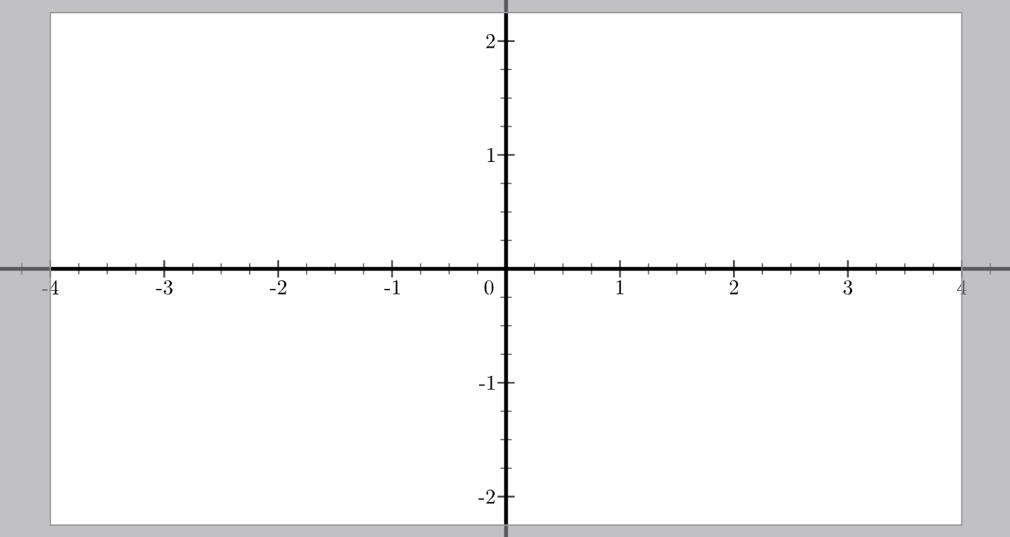
Also, whenever a function asks for a color, it means a vector of four numbers (red, green, blue, alpha), each in the range of 0 to 1. To actually change the color of most meshes, you'll likely have to click on the <> icons next to color (see functor modes from previous lesson).
3.3 Meshes
DEFINITION A mesh is a connected* collection of dots, lines, and triangles. Each vertex has an associated color.
Primitive meshes are meshes that you can create directly (i.e. no prerequisite meshes needed). Some common examples:

- Circle is a simple geometric circle
- Tex can be used to render latex equations
- ColorGrid displays a bunch of rectangles according to a user-provided color function
- Axis2d is helpful in graphing scenes
Operator meshes (or more accurately, operators on meshes) take in one or more mesh-trees, and spit out a new a mesh-tree. Here are a few examples (you can find more in the documentation section):
- Shifted translates a mesh-tree by a certain delta
- Rotated rotates a mesh-tree along a given axis
- Centered translates the mesh-tree so that its center is placed at the given location
- PointMapped moves every single vertex in the mesh-tree to a new point using the given transformation function
- XStack arranges a series of meshes in the x direction
3.4 Mesh-Tree
Typically, we want to consider not just a single mesh, but a collection of them. This is where mesh-trees come in.
DEFINITION A mesh-tree is defined recursively. A mesh is a mesh-tree. A vector of mesh-trees is a mesh-tree.
Informally, we can think of a mesh-tree as just a list of meshes, that might have similar such lists inside of them. Example (assuming all the variables are meshes): {mesh_a, mesh_b, {{{{mesh_c}}}}, {mesh_d, {mesh_e}}}.
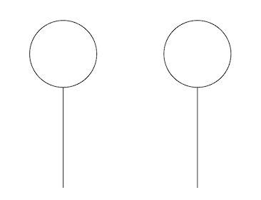
REMARK To those who ask why we can't just use a flat vector, note that mesh-trees allow us to be sloppy with the structure of our variables, which makes programming much easier. It also provides some sort of abstraction where we can ignore the exact details of how functions structure their returned mesh-trees. For instance, notice the following simple example where the baloons vector is not a flat list:
func Balloon(position) = identity:
    let head = Circle:
        center: position
        radius: 0.5
        tag: {}
        stroke: BLACK

    let string = Line:
        start: head
        end: vec_sub(position, {0, 2, 0})
        tag: {}
        stroke: BLACK

    element: {head, string}

tree balloons = {}
balloons += Balloon:
    position: {-1, 0, 0}
balloons += Balloon:
    position: {1, 0, 0}

/* at this point balloons has the following structure: */
/* {{head_1, string_1}, {head_2, string_2}} */

p += Set:
    vars&: balloons
IMPORTANT Most library functions dealing with meshes allow you to input an entire mesh-tree. Operations on a mesh-tree simply operate on all the meshes contained within the tree.
3.5 (Optional) Why meshes?
In many computer graphics contexts, Bezier curves are used instead of the meshes we just talked about. The decision to use meshes primarily comes as a way to make all screen objects the same type, which is harder to do with Bezier curves. On the other hand, there are instances where meshes are much less smooth than Bezier curves, which is undesirable.
For instance, the following would require many Bezier curve objects, but can be done in a single mesh.
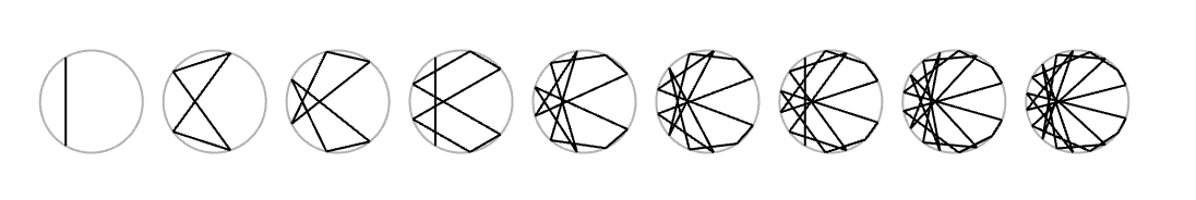
3.6 Complex Example
To create complex scenes, you have to think about the constiuent parts, and how each own can be written as a pipeline of primitives and operators. Here's an example and the result:
Code:
/* helper function, takes in number of lines and radius */
func Cardiod(n, r) = identity:
    var ret = {}
    ret += Circle:
        center: ORIGIN
        radius: r
        tag: {}
        stroke: LIGHT_GRAY

    func theta_to_point(theta) = {r * cos(theta), r * sin(theta), 0}
    for i in 0 :< n
        let next = mod(i * 2, n)
        let org_theta = TAU * i / n
        let new_theta = TAU * next / n
        ret += Line:
            start: theta_to_point(org_theta)
            end: theta_to_point(new_theta)
            tag: {}
            stroke: BLACK

    element: ret

/* create 9 raw cardiods */
let raw_cards = map:
    v: 1 :< 10
    f(x): Cardiod:
        n: 2 * x + 1
        r: 0.25

/* use operators to position them */
tree cards = Centered:
    /* for simple operators it can be okay to use functions */
    mesh: XStack(raw_cards)
    at: ORIGIN

p += Set:
    vars&: cards
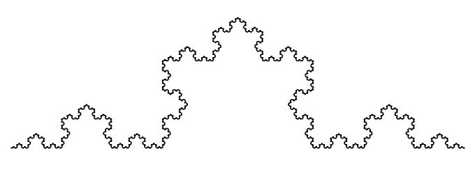
3.7 More Examples!
Here's the code for a Koch Curve and the result:
func move(start, mag, rotation) = identity:
    let delta = {mag * cos(rotation), mag * sin(rotation), 0}
    element: vec_add(start, delta)

func KochCurve(level, start, length, rotation) = identity:
    var ret = {}
    if level > 0
        var pos = start
        var rot = rotation
        ret += KochCurve:
            level: level - 1
            start: pos
            length: length / 3
            rotation: rot

        pos = move(pos, length / 3, rot)
        rot += PI / 3
        ret += KochCurve:
            level: level - 1
            start: pos
            length: length / 3
            rotation: rot

        pos = move(pos, length / 3, rot)
        rot += 4 * PI / 3
        ret += KochCurve:
            level: level - 1
            start: pos
            length: length / 3
            rotation: rot

        pos = move(pos, length / 3, rot)
        rot += PI / 3
        ret += KochCurve:
            level: level - 1
            start: pos
            length: length / 3
            rotation: rot
    else
        ret += Line:
            start: start
            end: move(start, length, rotation)
            tag: {}
            stroke: BLACK

    element: ret

let l = 4
tree k = KochCurve:
    level: 5
    start: {-l / 2, 0, 0}
    length: l
    rotation: 0

p += Set:
    vars&: k
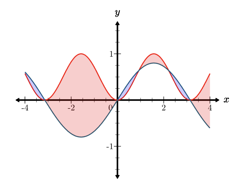
Here's one for the difference between two functions
func f(x) = sin(x) ** 2
func g(x) = sin(x) * 4 / 5

tree scene = {}
scene += Axis2d:
    center: ORIGIN
    x_unit: 2
    x_rad: 4
    x_label: "x"
    y_unit: 1
    y_rad: 1.5
    y_label: "y"
    grid: off
    tag: {}
    color: BLACK

var graphs = {}
graphs += ExplicitFunc:
    start: -4
    stop: 4
    f(x): f(x)
    tag: {}
    stroke: RED

graphs += ExplicitFunc:
    start: -4
    stop: 4
    f(x): g(x)
    tag: {}
    stroke: BLUE

graphs += ExplicitFuncDiff:
    start: -4
    stop: 4
    f(x): f(x)
    g(x): g(x)
    tag: {}
    pos_fill: {1,0,0,0.2}
    neg_fill: {0,0,1,0.2}

/* helps morph meshes into the axis space */
scene += EmbedInSpace:
    mesh: graphs
    axis_center: ORIGIN
    x_unit: 2
    y_unit: 1
    z_unit: 1

p += Set:
    vars&: scene
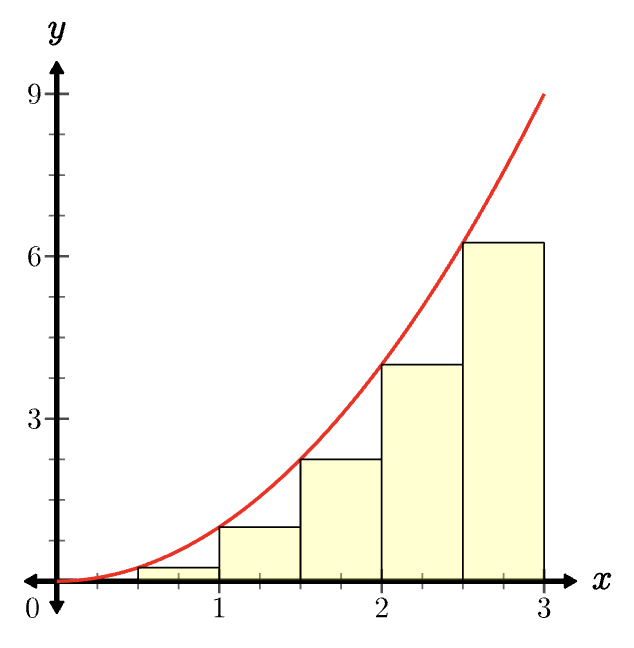
Riemann rectangles
func LRAM(start, stop, n, q(x)) = identity:
    var ret = {}
    let delta = (stop - start) / n
    for i in 0 :< n
        let x_start = start + delta * i
        let x_end = x_start + delta
        let val = q(x_start)
        ret += Rect:
            center: {(x_start + x_end) / 2, val / 2, 0}
            width: delta
            height: val
            tag: {}
            stroke: BLACK
            fill: {1,1,0,0.2}

    element: ret

func q(x) = x * x

tree scene = {}
scene += Axis2d:
    center: {-1.5,-1.5,0}
    x_unit: 1
    x_min: 0
    x_max: 3
    x_label: "x"
    y_unit: 3
    y_min: 0
    y_max: 9
    y_label: "y"
    grid: off
    tag: {}
    color: BLACK

var graphs = {}
graphs += ExplicitFunc:
    start: 0
    stop: 3
    f(x): q(x)
    tag: {}
    stroke: RED
graphs += LRAM:
    start: 0
    stop: 3
    n: 6
    q(x): q(x)
scene += EmbedInSpace:
    mesh: graphs
    axis_center: scene[0].center
    x_unit: 1
    y_unit: 3
    z_unit: 1

p += Set:
    vars&: scene
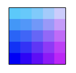
The color grid from before
tree grid = ColorGrid:
    x_min: 0
    x_max: 1
    y_min: 0
    y_max: 1
    x_step: 0.2
    y_step: 0.2
    tag: {}
    color_at(pos): {pos[0], pos[1], 1, 1}
    stroke: BLACK

p += Set:
    vars&: grid
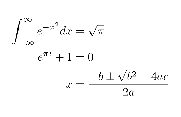
Some famous LaTeX equations
tree equations = Text:
    var str = "\begin{align*}"
    str += "\int_{-\infty}^{\infty}e^{-x^2}dx &= \sqrt{\pi} \\"
    str += "e^{\pi i} + 1 &= 0 \\"
    str += "x &= \frac{-b \pm \sqrt{b^2 - 4ac}}{2a} \\"
    str += "\end{align*}"
    text: str
    scale: 0.75
    stroke: CLEAR
    fill: BLACK
equations = Centered:
    mesh: equations
    at: ORIGIN

p += Set:
    vars&: equations
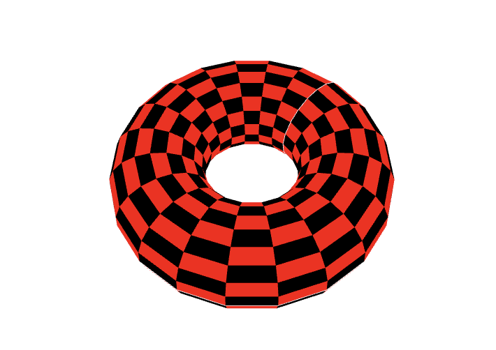
Torus (with some camera work)
/* checkerboard */
let uv_base = ColorGrid:
    x_min: 0
    x_max: 1
    y_min: 0
    y_max: 1
    x_step: 0.05
    y_step: 0.05
    tag: {}
    color_at(pos): identity:
        let r = round(pos[0] / 0.05)
        let c = round(pos[1] / 0.05)
        var col = BLACK
        if mod(r + c, 2)
            col = RED
        element: col

let r1 = 1
let r2 = 0.5
tree torus = PointMapped:
    mesh: uv_base
    point_map(point): identity:
        let u = point[0] * TAU
        let v = point[1] * TAU
        let x = (r1 + r2 * cos(v)) * cos(u)
        let y = (r1 + r2 * cos(v)) * sin(u)
        let z = r2 * sin(v)
        element: {x,y,z}

p += Set:
    vars&: torus
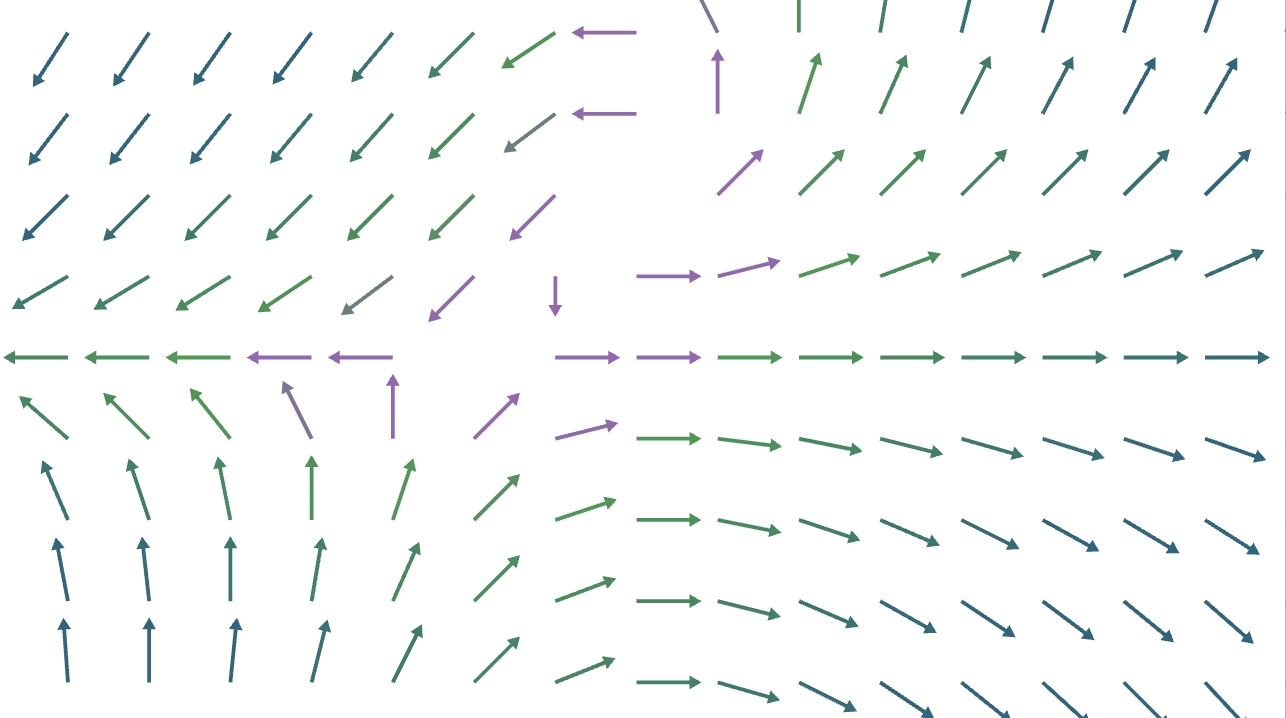
Vector Field
/* somewhat hard coded for sake of example */

let min_norm = 1
let max_norm = 5
let max_scaled_norm = 0.4

var gradient = {:}
gradient[min_norm] = PURPLE
gradient[1.5] = GREEN
gradient[max_norm] = BLUE
let gradient_c = gradient

func VectorField(f(x,y)) = Field:
    x_min: -4
    x_max: 4
    y_min: -2
    y_max: 2

    mesh_at(pos): Vector:
        var raw_delta = f(pos[0], pos[1]) + 0

        let mag = norm(raw_delta)
        let color = keyframe_lerp(gradient_c, mag)

        var scale = 1
        if mag > max_scaled_norm
            scale = max_scaled_norm / mag
            raw_delta = vec_mul(scale, raw_delta)

        tail: pos
        delta: raw_delta
        tag: {}
        stroke: CLEAR
        fill: color

tree field = VectorField:
    f(x, y):  {-y+x+1,x*y}

p += Set:
    vars&: field
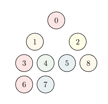
Tree (Graph Theory)
func tint(color) = {color[0], color[1], color[2], 0.1}
func Node(position, color, label) = identity:
    var ret = {}
    ret += Circle:
        center: position
        radius: 0.2
        tag: {}
        stroke: BLACK
        fill: tint(color)

    ret += Number:
        value: label
        precision: 0
        scale: 0.5
        tag: {}
        stroke: CLEAR
        fill: BLACK

    ret[1] = Centered:
        mesh: ret[1]
        at: position

    element: ret

/* we can add edges as well using a technique in lesson 7 */
/* without that, they are hard to add unfortunately */
func Tree(adj, colors, curr, position) = identity:
    var ret = {}
    ret += Node:
        position: position
        color: colors[curr]
        label: curr

    var children = {}
    for child in adj[curr]
        children += Tree(adj, colors, child, position)

    /* position */
    children = XStack:
        mesh_vector: children
        align_dir: UP

    ret += children
    ret = Stack:
        mesh_vector: ret
        dir: DOWN
        align: center

    element: ret

/* adjacency list */
let adj = {{1,2}, {3, 4}, {5, 8}, {6}, {7}, {}, {}, {}, {}}
let colors = {RED, ORANGE, YELLOW, RED, GREEN, BLUE, RED, BLUE, ORANGE}
tree graph = Tree:
    adj: adj
    colors: colors

    /* 0 is root */
    curr: 0
    position: {0,1,0}

p += Set:
    vars&: graph
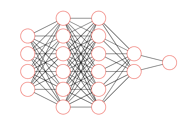
Neural Network
func NeuralNetwork(layer_counts) = identity:
    var layers = {}
    var edges = {}

    var last_layer = {}
    for i in 0 :< len(layer_counts)

        var new_layer = {}
        for j in 0 :< layer_counts[i]
            new_layer += Circle:
                center: {0, 0, 0}
                radius: 0.2
                tag: {}
                stroke: RED
                fill: WHITE
        new_layer = YStack(new_layer)
        new_layer = Centered:
            mesh: new_layer
            at: {i, 0, 0}

        layers += new_layer

        for prev in last_layer
            for curr in new_layer
                edges += Line:
                    start: prev
                    end: curr
                    tag: {}
                    stroke: BLACK

        last_layer = new_layer

    element: Centered:
        mesh: {edges, layers}
        at: ORIGIN

tree nn = NeuralNetwork:
    layer_counts: {4, 6, 6, 2, 1}

p += Set:
    vars&: nn
Look at more examples over here
3.8 Practice
Finally, you can try playing around with Monocurl! We still can't do animations yet, but as a challenge, try creating the following:
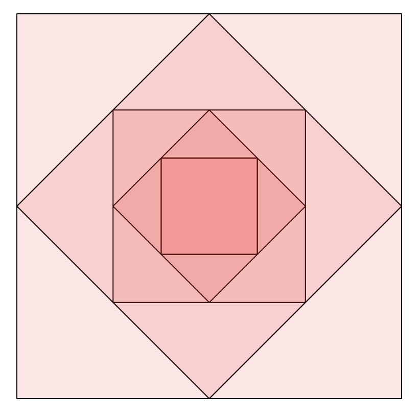
Hint, you can make the previous using just the following three meshes and operators (and a bit of math):
First get the placements right, then aim for the colors.
3.9 Conclusion
REMARK This sections covered the basics of meshes. The point isn't that you know all meshes by now, but rather you have a good enough idea that it's easy to learn new ones. We definitely recommend going to the docs page and exploring existing options. In particular, look out for the ones with a star, as those are pretty useful.
Also, hopefully you can see the importance of creating your own functions from the very few examples we gave. As scenes get more complex, functions are of even more importance.
3.10 (Optional) Remarks
REMARK I dont really like positioning (and think it gets pretty redundant), and there are some stuff to be improved. But overall, I think meshes are good enough for the beta release.